- 2020/10/28

In this post we present the main steps required to create a custom utility in OpenFOAM.
Step 1) Defining utility objectives
When creating a custom utility, we start by defining its inputs, desired outputs and search if in the available source code exists a utility that offers similar outputs.
Input: surface patch provided by snappyHexMesh
Output: provide the center point of the surface patch and the vector passing through the center point and normal to the surface.
To get the center of the patch, we can use the approach represented in the following picture:
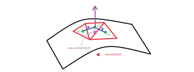
The patch will be discretized by snappyHexMesh in a series of faces (the red triangles), and for each face we can retrieve its center coordinates. Therefore we can implement the following approach:
- Compute the average of the centers of each face belonging to the patch (the red triangle in the picture). This will provide the “centerPatch” point that if the surface is flat, it will be the center of the patch straightaway. But if the surface is curved, then it will be outside of the patch surface, and we need to get its projection on the surface (represented by “new centerPatch” in the picture).
- Then we can compute the “new centerPatch” coordinates by averaging the 3 centers faces “p1”, “p2”, “p3” that are the nearest to “centerPatch”.
- “p1”, “p2”, “p3” will also provide us 2 non parallel vectors “a” and “b” locally coplanar to the surface (vector a and b in the picture). By computing the cross product of axb we can get the normal vector at “new centerPatch” point.
Step 2) Gathering useful OpenFOAM source code snippets
To implement the above approach, first we need to understand how to retrieve the face center and compute their average to get “centerPatch”. One of the existing utility that we can take as starting point for our code is “patchAverage.C”. Another interesting file from which we can get useful definition is “Test-mesh.C”. From Test-mesh.C we can get some useful definitions:
- C() gives the center of all cells and boundary faces
- V() gives the volume of all the cells.
- Cf() gives the center of all the faces.
We start by copying all the patchAverage directory (including its nested Make directory required to compile the code) into our home directory. There we rename the directory to ““normalCenterCalc”. Then enter the directory and rename “patchAverage.C” to “normalCenterCalc.C”. Also in normalCenterCalc/Make/files substitute “patchAverage” with “normalCenterCalc” so that you have :

In this way we have a little platform that we can use to test, assemble and compile our code.
Step 3) Assembling the code and compiling
Source OpenFOAM:

Enter your custom code directory and compile it:

In the beginning it will behave just like patchAverage.C. But from there we will insert code from Test-mesh.C and start to do simple tests. Like for example choosing a simple case, like the “incompressible/icoFoam/cavity” tutorial. The simpler the mesh, the better it is to debug your code. For example we can start by testing simple instructions like

this will output to terminal the list of the center of faces. Then we can build longer expressions and for example narrowing the output to list face centers only belonging to a certain patch. The following syntax
will provide the list of face centers for patchI only. To get the center of the patch we then just need to sum all the coordinates of the centers of faces using the function “gSum”:![]()
and divide that sum by the number of faces present in the patch, number that can be obtained with the following syntax, where we append the method “size()”:
Therefore the centerPatch coordinates given by [sum of faces centers coordinates]/[number of faces of the patch] in OpenFOAM syntax becomes: ![]()
Source code highlights
You can download the full code of the normalCenterCalc.C from this link https://github.com/alsdia/normalVectorCalculator. Below we copy just some excerpts from the source code to explain some relevant passages:
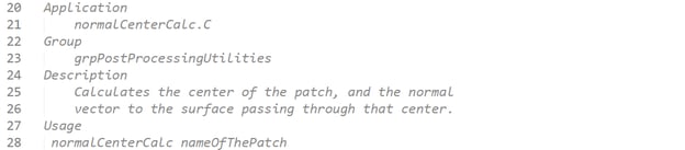
In the top comment section lines 20-28 we update the application name, and the description of the utility:
Then, in lines 30-34 follows the include list where are included the Headers files “*.H” required by our custom utility. In this way, when we compile the utility, the preprocessor will copy the entire contents of those header files into our program: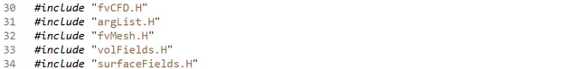
Then all the section from line 38 to 51 is just following the same approach of patchAverage.C, but in line 49 we comment “//(timeDirs[timeI], timeI);” and use instead “runTime.setTime(0,0);” so that the utility compute only for the 0 directory and doesn’t repeat the computation for all the following time directories:
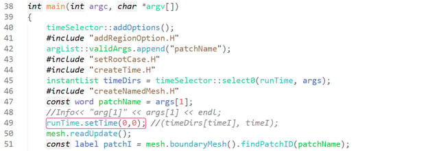
Moreover in line 47 “const word patchName = args[1]; // args[2];” we set args[1] since we just need to process one patch, so we just need 1 argument.
In line 63 we compute the “centerPatch” as explained in the previous “Step 3)” section :
![]()
This value is backup in “centerPatchOrg” in line 68. Then we proceed to search for the 3 center faces (from the mesh.Cf().boundaryField()[patchI].size() list) that are the nearest to “centerPatchOrg”.
![]()
To get those nearest 3 centers faces ( represented by p1, p2, p3 in the picture below) we will do a for loop for each of the faces of the mesh and save the coordinates of p1, p2, p3 in 3 vectors centerP1, centerP2, centerP3.
In line 75 we initialize the variables first, second, third that we use to save the distances between p1, p2, p3 and centerPatch.

In line 80 we initialize the vector to save the nearest 3 points coordinates to centerPatch:

Then we start the for loop and for each faces center belonging to the patch (line 84) and save the distance between the i face center and centerPatch in the distanceSquare variable (line 87):
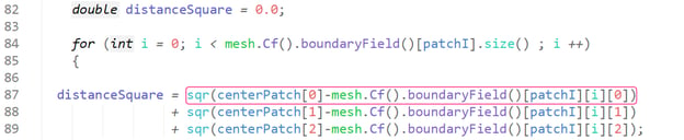
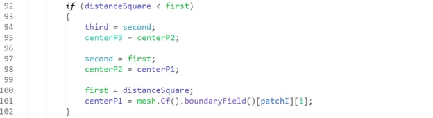
sqr(a) in line 87 means a*a. Since we just want to know the shorter distance is enough to compute the square of the distance, we don’t need to perform a sqrt to get the actual distance. distanceSquare in line 82 is initialized with the minimum value zero. Once the loop starts, distanceSquare will get the value of the square of the distance between the i-th face and centerPatch. If its value is smaller than any value found before, then we execute the section of code lines 94-101 where the 2nd nearest point becomes the third, the old first become the second and the first point become the new i-th found face center:
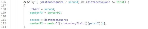
On the contrary if distanceSquare is between the first and second previous found nearest centers, then we need to update second and third as shown in the lines 106-113:
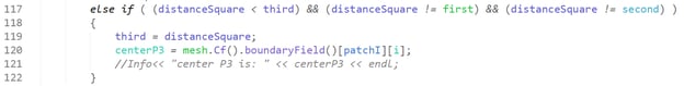
And if the found distanceSquare is between the second and third previously found nearest centers, then we just need to update the third centerP3, while centerP1 and centerP2 keep the same values, this is done in lines 117-122:
Once the for loops completes we have finally the coordinate of the 3 nearest face centers p1, p2, p3 and we can use them to compute the cross product to get the normal vector to the patch as shown in line 132:

On line 136 we normalize the normal vector using the “mag()” function :
![]()
Then line 139 performs the average of the coordinates of p1, p2, p3 to get a good approximation of a center patch belonging to the patch surface even in case of open non planar surfaces.

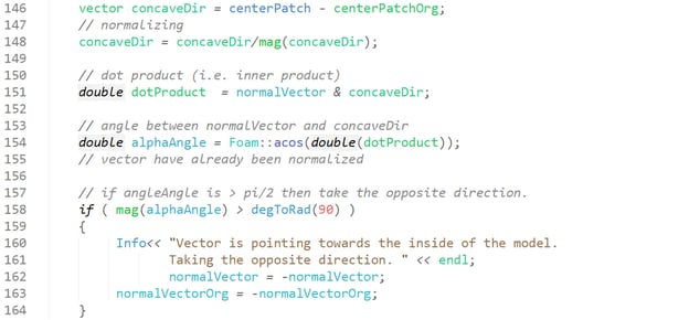
In the lines 146-164 we perform an additional test to know which is the convex and concave side of the patch. We compute the dot product between the "normalVector" and the vector "centerPatch-centerPatchOrg". If the angle between "normalVector" and "centerPatch-centerPatchOrg" is greater than pi/2, it means the "normalVector" is pointing towards the "inside" concave side of the patch, and therefore we must invert the direction:
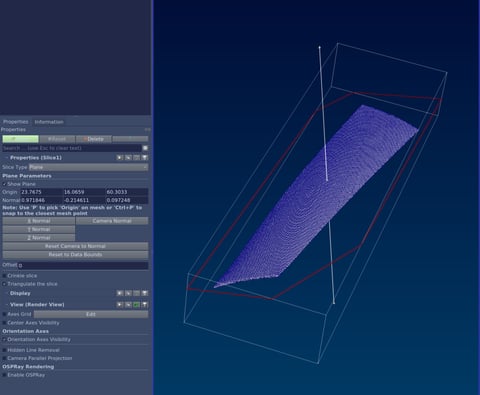
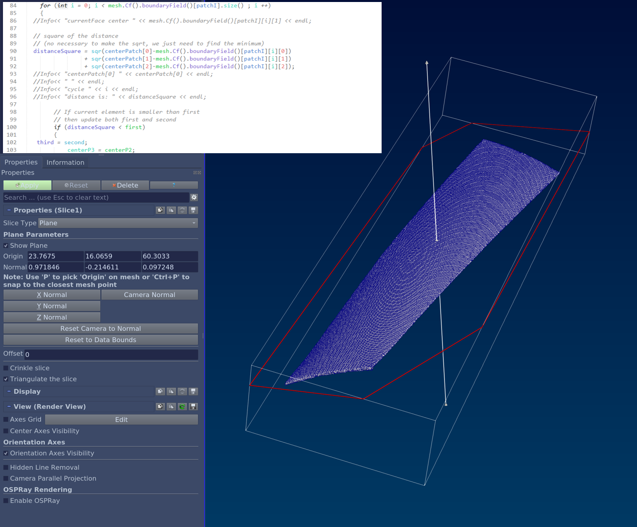
Step 4) Validating the code with test case
We take a simple geometry and mesh it with snappyHexMesh. Then we process the patch with normalCenterCalc and verify in Paraview that center and normal vector are correct. The code gives us as output “The normal vector to the patch is: (0.97184614 -0.21461106 0.097247959), Center of the patch is: (23.767507 16.065936 60.303342)”. By putting these numbers into the Origin and Normal entries in the “Slice” filter property panel of Paraview, we can clearly see that the estimation is correct.