Falcon Heavy Rocket Simulation with OpenFOAM

ROCKETS SIMULATIONS

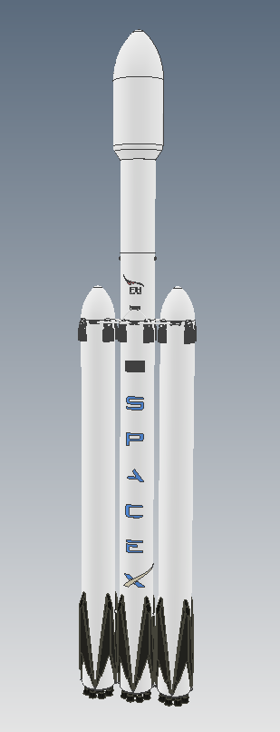
Objective: take Falcon heavy rocket model and launch it with sonicFoam with k-epsilon as turbulence model.

Geometry

We can download the STLs from https://grabcad.com/library/spacex-falcon-heavy-space-rocket-1 

For the CFD simulation, we can simplify a little bit the geometry in Viscart:

Also we need to rescale the geometry in meters.

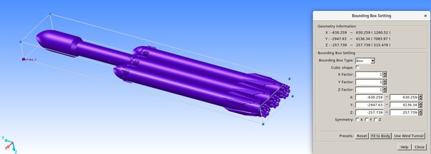
The original height of the model is 2947.63 + 4136.34 = 7083.97 -> these are cm, we need to rescale the model with 1/100, so that the height becomes 70.83 meters ~ similar to the 70m total height specified in  https://en.wikipedia.org/wiki/Falcon_Heavy 

Once scaled, with the filter “split selected geometry” we can disassemble the STL surface into 400 surfaces, so to delete some of the details and merge some patches. Also we add outlet patches to each of the 27 nozzles of the Merlin engines.  

Meshing

We export the new simplified STL from Viscart and import into VisualCFD. The rocket is 70.8m tall. To avoid having shock waves be reflected from the outer wall of the bounding box, we will set the bounding box walls 70meters apart from the side walls of the boosters. The inlet is 70 meters from the flare and the outlet is 140m from the nozzles. In the following picture is shown the overall domain dimension:

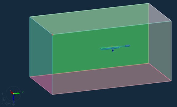
The diameter of the nozzle at the outlet section is 0.92m.

Mesh Parameters settings: we would like to have the highest refinement around the nozzles. Since the diameter is 0.92m, we can choose a level0 cell size of 2.5m and then impose a refinement level of 7 near the nozzles, so that the cells adjacent to the engines are 0.0195m (that is 0.92/0.0195 ~ 47 cells along the nozzle diameter). Below the settings used in Visual CFD snappyHexMesh parameters:

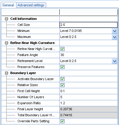
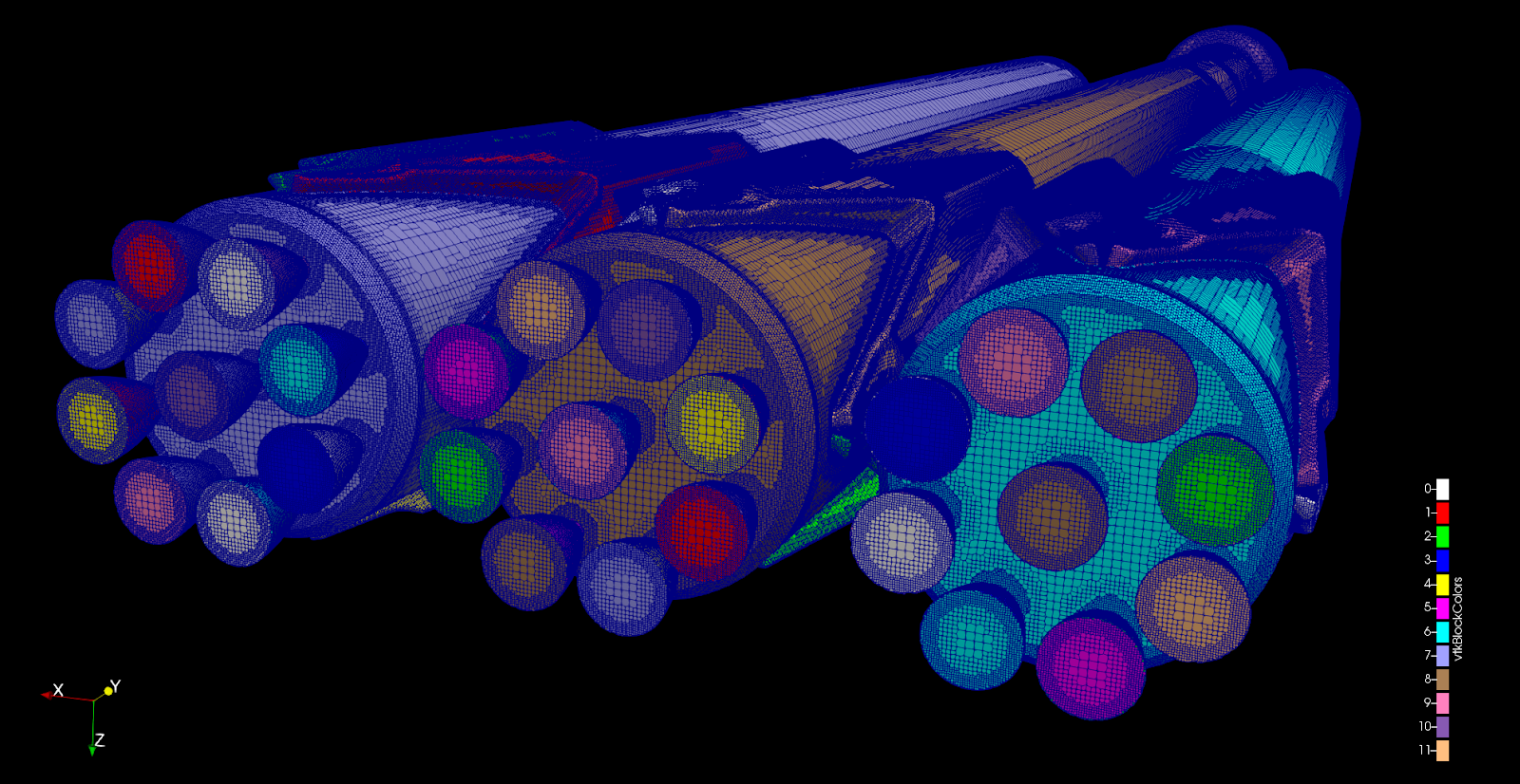
With the above refinement settings we get a mesh of around 10 millions cells:

Layer mesh : cells:9877403  faces:31446263  points:11806484

Boundary conditions

As a reference case to set our boundary conditions and numerical schemes, we follow the tutorial case tutorials/compressible/sonicFoam/RAS/nacaAirfoil.  Like in the tutorial the inlet boundary condition are set as follows:

"inlet.*"

        {

             type            supersonicFreestream;

             pInf            $pressure;

             TInf            $temperature;

             UInf            $flowVelocity;

             gamma               1.4;

             value           $internalField;

        }

At sea level, at a temperature of 21 degrees Celsius (70 degrees Fahrenheit) and under normal atmospheric conditions, the speed of sound is 344 m/s, so let’s suppose to fly at Mach 2 = 344* 2 = 688, and set the Uinf with flowVelocity (0 -688 0).

Concerning the velocity outlet at the nozzle, we need to take into account the ISPof the Merlin Engine. As explained in https://en.wikipedia.org/wiki/Specific_impulse we can compute the outlet velocity of the engine by using the formula:

V_outlet = Isp * g = 282 * 9.81 = 2766.4 m/s

Where Isp = specific  impulse of the engine, and g is the Earth gravity.  This means that in the engine region we are at around Mach 8, hypersonic regime where sonicFoam will likely be unable to give accurate results. Let’s pull ahead anyway to see how far we can go.

Results

The analysis remains stable only in the initial time steps as shown in the pictures below:

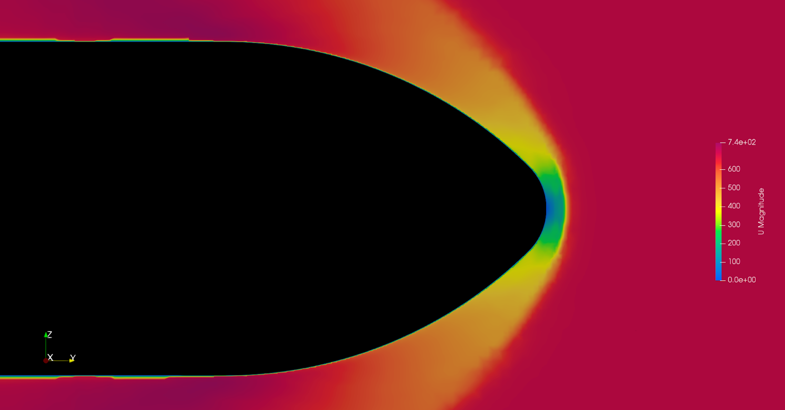
Velocity field around the flare

After some iterations, the velocity in the region near the nozzle of the engines becomes unbounded and the analysis crashes. After several attempts with different mesh refinements and tailoring the numerical schemes we were not able to completely solve all convergence issues, but at least the analysis was stable for the first few fractions of second:

Pressure field on the Falcon heavy walls

Pressure field cut plane

Velocity field cut plane

The case will then show convergence issues around 0.004s in the nozzle region where the speeds are not anymore in the suitable range for  the sonicFoam solver.

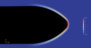
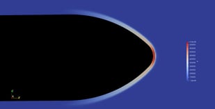
Still if we compare the pictures below we can see that qualitatively the overall velocity field of the exhausts gases look similar to the experimental field where few meters from the nozzle we can see that hourglass shape of the plume where the gases are pinched by high ambient air pressure:

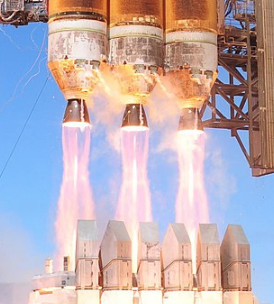
Since we are at sea level, the Exit Pressure of exhaust (Pe) is smaller than the Ambient pressure (Pa), we are in a “over expanded” condition [case (a) left in the following picture]

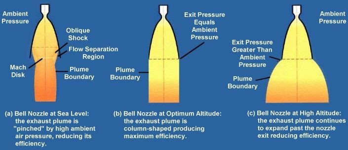
[source https://www.thespacetechie.com/the-shape-of-rocket-exhaust/]